

How to Play
The story
Guroble has just set up business in Burritoville! Guroble needs your assistance to plan where to place its burrito trucks to serve hungry customers throughout the city and maximize its profit. Truck placement has to be carefully planned, because every truck has a cost, but its ability to earn revenue depends on how close it is to potential customers. On some days, special events increase the demand in some regions of the city; on other days, the weather affects customers’ willingness to walk to a burrito truck. Help Guroble succeed by playing the Burrito Optimization Game!
The Gameboard
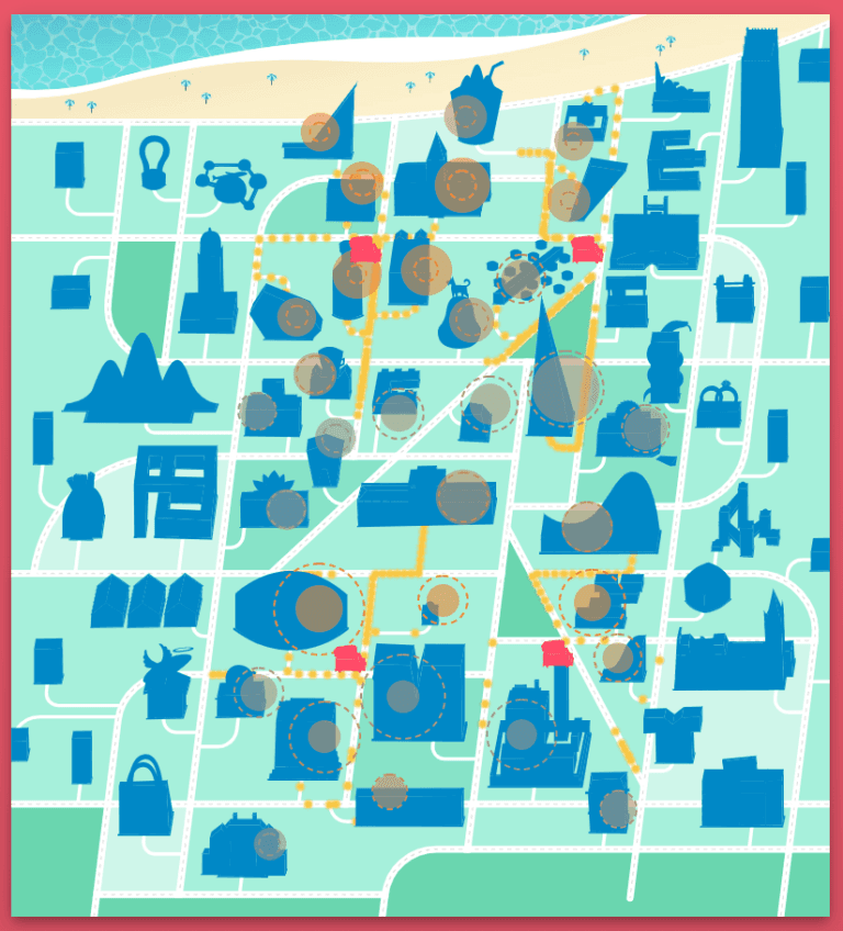
The gameboard is a map of Burritoville, full of potential customers who are hungry for burritos. Customers are located in buildings throughout the city. Buildings that have interested customers today have a demand marker: a circled number, which indicates the maximum number of customers you can win on that day. But you might not win all of them! Customers are only willing to walk so far to a burrito truck, and the actual number of customers you win from a building is smaller the farther away the truck is from the building. If the nearest truck is too far away, you won’t win any customers from that building. Once you have placed a truck, you will see an animation of the customers walking from buildings to the truck.
Trucks have unlimited capacity—each truck can serve an unlimited number of customers.

The percentage of customers served at a building is indicated by a partially or a totally filled circle around the demand marker. You can hover your mouse over a building to find out exactly how many customers your current trucks have won from that building.Trucks have unlimited capacity—each truck can serve an unlimited number of customers.

Your job is to choose where to locate trucks. Trucks can only be placed at certain spots in the city, which will be highlighted when you are dragging a truck onto the map.

To place a truck, select the truck icon from the lower menu bar and drag it to one of the highlighted spots. You can move a truck from one spot to another one by dragging and dropping it. You can remove a truck from a location by dragging it from the map to the trashcan icon on the lower menu bar.

Gameplay
Before each day, a newsfeed will describe what’s happening on that day and list the revenue and cost parameters for the day. For example, on Round 1, Day 1, each truck that you place will cost ₲250, and each burrito that you sell (each customer that you win) will cost ₲5 in ingredient costs but earn you ₲10 in sales revenue. (₲ is the symbol for Gurobucks. Naturally.)
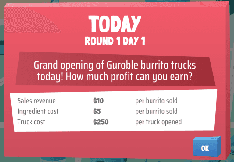
After you click OK on the newsfeed, you will start placing trucks on the map to serve customers. Your profit for the day is calculated using a simple formula:
Today's Profit = Sales Revenue - Ingredient Cost - Truck Cost
You can see the current values of Today’s Profit, Sales Revenue, Ingredient Cost, and Truck Cost on the lower toolbar.

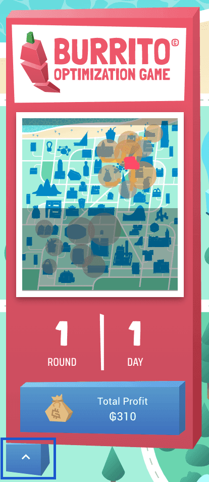
The sidebar on the left-hand side of the screen shows the Total Profit—the sum of the daily profits from all of the days you have played so far (including the current day).

Also on the sidebar is the minimap, which shows a birds-eye view of the city. On the minimap, you will not see the demand numbers, but circles representing them: the larger the dot, the more customers at that building. The circles change color depending on how many customers you have won from that building: more orange means you have won a larger percentage of the customers, more gray means a smaller percentage.

You can minimize the sidebar by clicking the button below it. (This makes it easier to view and access some parts of the map.)
You can zoom in or out of the map using the magnifying glass icons on the top right corner of the gameboard.

If you want to remember today’s newsfeed, you can click on the News button on the top right corner of the gameboard.

If you want to turn on or turn off the sound in the game, you can click on the audio button on the top right corner of the gameboard.

BONUS: If you want to download the underlying data for a particular day’s problem, you can click on the red download button on the top right corner of the gameboard.

Finally, the Restart button on the bottom toolbar resets the game back to Round 1, Day 1, and the Exit button brings you back to the home page.
Finishing up a Day
When you are satisfied with your truck placements, click the Done button on the bottom toolbar.
NOTE: Until you click “Done”, you are still only planning your strategy to achieve optimal truck placement to meet customer demand. Consider your score finalized for the day once you click Done.

When you click Done, in addition to sizing up your solution, the game will find the optimal solution for the day by calling the Gurobi optimizer. You’ll see a screen that displays both solutions—yours and Gurobi’s—and compares their profits. How close can you get to Gurobi’s solution?
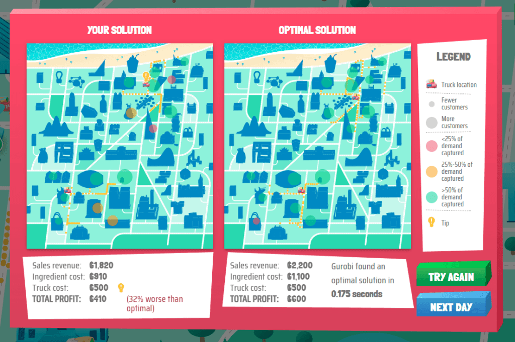
This map is similar to the minimap: The demand markers are replaced by filled circles whose size indicates the demand at each building, and the circles that are more orange mean you have won a larger percentage of the demand at that building, while those that are more gray mean you have won a smaller percentage.
(In Championship Mode, you’ll be able to see the optimal profit, but not the optimal solution. No peeking!)
Days and Rounds
The game is divided into rounds, and every round is divided into days. Each day brings a new wrinkle: for example, different customer locations, demand numbers, or cost parameters. Every day the map is empty of trucks and you have to start planning again.
In Round 2, you won’t know the exact demands—the numbers inside the demand markers are only forecasts of the demands. The actual demands are random. Your solution—and Gurobi’s—will be evaluated using the actual demands, but you won’t learn those until after you click Done.
Note: Gurobi’s solution (like yours) is optimized using the demand forecasts. But since both solutions are evaluated based on actual demands, it’s possible that your solution can be better than Gurobi’s, if you get a lucky set of random demands.
On some days during Round 2, you’ll see error bars telling you the range of values the actual demand will fall into. Sometimes these are symmetric, meaning the demand is equally likely to be greater than or less than the forecast—

—and sometimes they are asymmetric, meaning the demand is more likely to be higher or lower—

Technical note: If you’re interested, the demands follow a triangular distribution with minimum and maximum values equal to the end points of the error bars and mode equal to the forecast value. The mean of a triangular distribution with minimum a, maximum b, and mode c is (a+b+c)/3.
The maps that show your solution and Gurobi’s at the end of each day in Round 2 are similar to those in Round 1, except that each building also has a dashed circle that indicates the demand forecast. (The filled circles indicate the actual demand. Remember that your solution, and Gurobi’s, earn revenue and incur costs based on the actual demand, not the forecast.)
Championship mode
Championship mode offers a way to compete against your friends or colleagues while playing the Burrito Optimization Game. Championship mode is designed for classes, conferences, or other events. The event organizer will share a Match Code with you, which you will enter into the game, as well as your display name. Play the game as usual. Then, at the end of the Championship, you will see the rankings of top players and have the opportunity to enter your own display name onto the Scoreboard—if your solutions were good enough!
Note: Only use Championship mode if you were instructed to do so. If you are playing the game on your own, just click “Play the Game” to play in normal mode.
Optimal Solutions
Is the Gurobi solver trying all possible solutions?
No!
The map has 56 possible truck locations. That means there are 2^56 = 72,057,594,037,927,936 possible solutions—that’s 72 quadrillion! Even if your computer could evaluate, say, 1 billion solutions per second, it would take more than 2 years to find an optimal solution by checking them all. (Checking all of the solutions and picking the best one is an algorithmic approach called enumeration.) But Gurobi is solving the problem, optimally, in a second or two. Gurobi is doing something much smarter and faster than enumeration.
(Oh and by the way: If there were 100 possible truck locations, it would take more than 40 trillion years to find an optimal solution by enumeration. Gurobi could still do it in seconds.)
What is the Gurobi solver actually doing
The high-level version
When we built the game, we also formulated an integer programming (IP) problem that represents the task faced by the player: choosing where to locate trucks to maximize profit. Integer programming problems are mathematical objects that express a set of decisions, the benefits or costs of those decisions, and constraints on what is and isn’t allowed in those decisions.
Each “day” of the game has its own version of the IP. Gurobi takes that IP as an input and uses cutting-edge algorithms to solve it. The algorithms have sophisticated mathematical ways to detect whether a certain decision (e.g., a certain truck location) will be good or bad, and to eliminate huge portions of those 72,057,594,037,927,936 possible solutions without even having to look at them.
Integer programming problems, and the algorithms used to solve them, are central to the field of operations research (OR), and also have strong connections to computer science and mathematics.
The IP: Notation
Now let’s get into some more detail about the IP itself, for those who have an appetite for the math. (In addition to burritos.)
Let I denote the set of buildings (we’ll call them customers now) and let J denote the set of potential truck locations. Our IP uses the following notation for the parameters of the model. (These are the inputs, or data, for the model.)
di = demand for customer i∈I
cij = travel distance from customer i∈I to truck j∈J
αij = demand multiplier for customer i∈I and truck j∈J. This multiplier depends on the distance: the further a customer i is from a truck location j, the less willing the customer is to walk to the truck
f = fixed cost that Guroble has to pay for placing a truck at a potential location
r = revenue per burrito sold
k = ingredient cost per burrito sold
Our model also has decision variables. These are the unknowns, or the choices to be made by the decision maker (whether that’s Guroble planners or the optimization solver):
xj = 1 if we locate a truck at location j, and = 0 otherwise, for each j∈J
yij = 1 if the closest truck to customer i∈I is at location j∈J (i.e., if i is assigned to j), and 0 otherwise
Both xj and yij are binary decision variables. They must equal integers (thus, this is an integer program), and in particular they can only equal the integers 0 or 1. Having binary variables (or general integer variables) in the model makes the problem much more difficult to solve. If we had a model with only continuous variables (that is, a linear program (LP)), the problem would be much easier and quicker to solve. Then, why not use only continuous variables? The power of binary variables lies in that there are some decisions that have a discrete nature. For example, we can choose whether to place a truck at a certain location or not, but we cannot place only a fraction of a truck.
Once we know (via the binary variable) whether we place a truck at a certain location, we can use that variable to “turn on” costs or revenues. For example, since xj=1 if we locate a truck at location j and 0 otherwise, we know that fxj equals the fixed cost f if we locate at j, and equals 0 otherwise. And then the total amount Guroble spends on fixed costs is ∑j∈Jfxj.
Another use for binary variables is to express logical relationships. For example, if the inequality yij≤xj is true, it tells us that if there is no truck at location j (xj=0), then customer i cannot be assigned to location j (yij must =0). If we impose this inequality as a constraint, then we are telling the solver that this is a rule that solutions must follow; that is, we are telling the solver that it may not choose to assign a customer to a truck node if it has not also chosen to locate a truck at that node.
You’ll see both of these “tricks” (using binary variables to turn costs on or off, and using them to express logical relationships) in the IP formulation below.
The IP: Formulation
The IP can be formulated as follows:

The first line is the objective function—a mathematical expression for the quantity we are trying to maximize (in this case) or minimize. The objective function for the Guroble IP maximizes the total profit, which is computed as the total net revenue minus the total cost of placing all trucks. The net revenue is the sum of the revenue minus the ingredient cost over all burritos sold (using a trick like the one described above to “turn on” costs for the customer–truck assignments that are active).
The remaining lines are constraints—restrictions that we place on the solutions that the solver is allowed to choose.
The first set of constraints says that each customer i∈I may be assigned to at most one truck j∈J. (Otherwise, we could win each customer multiple times by placing multiple trucks, which is not what actually happens in the game and therefore not what we should allow in the model.) The second set of constraints says that a customer i∈I can only be served by a truck j∈J (yij=1) if there is a truck positioned at location j∈J (xj=1). This is the logical relationship “trick” described above. The last two lines say that the decision variables must be binary (as opposed to continuous/real-valued, or general integers).
Nearly all mathematical optimization problems—linear programs, integer programs, mixed-integer programs, nonlinear programs, etc.—have the same structure as the formulation above: an objective function that specifies what we want to minimize or maximize, and a set of constraints the limit the possible values for the decision variables.
The IP formulation above, plus the data (the actual lists of customers and potential truck locations, the actual values for the costs and revenue parameters, etc.), give us a complete mathematical representation of the Guroble problem that you solved (by hand and approximately). Gurobi or another optimization solver can take this formulation and the data, do its magic (well, its algorithm—see below), and return the optimal solution (quickly and exactly, at least to within a tolerance specified by the user).
By the way, the Guroble IP is a special version of the Uncapacitated Facility Location Problem, a well-known problem in Operations Research where, given a set of potential facility locations and a set of customers, the decision-maker has to decide which facilities to open and assign customers to be served by open facilities. The usual objective is to minimize the total fixed costs for opening depots plus the transportation costs. The Facility Location Problem example on the Gurobi website provides a detailed description of the problem, together with a Jupyter notebook modeling example.
The Algorithm
The algorithm that Gurobi uses for solving IPs is called branch-and-bound. First proposed by Ailsa Land and Alison Harcourt (née Doig) in the 1960s, this algorithm takes a “divide-and-conquer” approach to exploring the range of possible solutions.
In branch-and-bound, we begin with the original IP. Not knowing how to solve this problem directly, we remove (“relax”) all of the integrality restrictions. The resulting LP is called the LP relaxation of the original IP, and this problem is much easier to solve. If the result happens to satisfy all of the integrality restrictions, even though these were not explicitly imposed, then we have been quite lucky, and we are done. If not, we proceed to branching, that is, we create two subproblems as follows: Take a binary variable xj. In one of the subproblems, we fix xj=0, and in the other subproblem, we fix xj=1. Then we solve both subproblems separately by repeating the process of first solving the corresponding LP relaxation (now with an extra constraint imposed by the branching decision), and if the solution does not satisfy the integrality constraints, then we repeat the branching procedure until there are no more binary variables left in the problem. In this way, we create a branch-and-bound tree, in which every node corresponds to a subproblem. (We only talked about branching on binary variables for simplicity, but it is also possible to branch on general integer variables.)
You might have realized that if we only do branching, this would be very similar to simply enumerating all solutions to the problem. The missing key ingredient is bounding. The main insight in the branch-and-bound algorithm is that not all solutions have to be enumerated, because the solutions to the LP relaxations of the different nodes provide bounds that tell us the best possible objective value we can obtain if we continue exploring a certain part of the tree. If we have found a feasible solution satisfying the integrality constraints while exploring a different part of the tree (which happens very frequently in practice), then we can discard big parts of the branch-and-bound tree by using the LP relaxation bounds and save valuable computing time. If we keep track of the current best feasible solution as we explore the tree, we will reach a point where there are no more branches to explore. The current best feasible solution at that point will be optimal for the original problem.
Here we have only sketched the branch-and-bound algorithm. There are many decisions to be made in a smart implementation of branch-and-bound: Which is the best sequence to choose the variables on which to branch? Which algorithm do we use to solve the LP subproblems? Can we solve some of the subproblems in parallel? Besides making these decisions in a smart way, Gurobi also applies presolve, cutting planes, heuristics, and parallelism, among other advanced techniques, to speed up the search process even more. The article Mixed-Integer Programming (MIP) – A Primer on the Basics gives an overview of these details.
Is it only for burritos?
Optimization is definitely not only limited to burritos! Integer programming (IP) and related areas like linear programming (LP), nonlinear programming (NLP), and mixed-integer nonlinear programming (MINLP) are enormously useful in practice. Optimization is used to solve complex, real-world problems in a wide variety of areas such as supply chain optimization, health care, electricity distribution, airport and aircraft operations, scheduling, personnel planning, marketing, and finance.
While playing the Burrito Optimization Game, you probably realized that solving optimization problems manually might be doable for very small scenarios, for example when there are only a few possible places to locate trucks. In that case, you might have obtained an optimal solution by trial and error. However, as the size of the problem grows, it becomes impossible to compute an optimal solution by hand. This is even more difficult if the input data are uncertain (random), which often happens in real applications. The power of integer programming (and related areas) lies in the fact that, once you know how to model your problem, you can optimize it using a general-purpose solver. Moreover, mathematical models provide great flexibility because changes in the input data are usually easily applied to the model, which can then be once again fed to the solver.
Gurobi’s case studies show several examples where optimization has made a big difference in real business cases.
The buildings
Pipe Benders: Benders decomposition is a technique for solving large-scale optimization problems that have a certain type of structure.
Traveling Salesperson Agency: The Traveling Salesperson Problem (TSP) is one of the most important problems in optimization. (The TSP can also be used to make art!).
ReLU Realty: Rectified Linear Unit (ReLU) is one of the most common activation functions for neural networks.
Cutting Stock Atelier: The cutting-stock problem is a classic optimization problem that aims to cut a large piece of “stock” (e.g., a roll of paper or metal) into standard-sized pieces while minimizing waste. It was one of the first applications of the column generation method of optimization.
Gaussian Mixture Shakes & Smoothies: A mixture model is a statistical model of a population (e.g., house prices) that consists of multiple subpopulations (e.g., different neighborhoods), each with its own probability distribution. Gaussian mixtures are a common type of mixture model.
Gu Library: Dr. Zonghao Gu is the Chief Technical Officer and a co-founder of Gurobi Optimization. The Gu Library in Burritoville is inspired by a building at Georgia Tech, where Dr. Gu received his PhD degree.
Barrier Fencing: Barrier methods are another name for interior-point methods, a type of algorithm for solving linear and some nonlinear optimization problems by exploring the interior of the feasible region. (In contrast, the simplex method explores the corners of the feasible region.)
Poisson Distribution Fish Market: The Poisson distribution is a probability distribution that is often used to represent random arrivals to a queuing system. (It is named after Siméon Denis Poisson, whose surname means “fish” in French.)
The Euclidean Space: Euclidean space is the type of space used in classical geometry (that is, the geometry you learned in high school). It is also fundamental to how we represent and solve optimization problems.
The Analytic Center: The analytic center of a convex polygon is a point inside the polygon that maximizes the product of distances to the sides. It has important connections to certain types of optimization algorithms.
LP Relaxation Spa: The LP relaxation of a mixed-integer programming (MIP) problem is the problem obtained when “relaxing” (that is, disregarding) the constraints requiring the variables to be integers. LP relaxations play a fundamental role when solving MIPs using the branch-and-bound algorithm.
Rothberg Tower: Dr. Edward Rothberg is the Chief Executive Officer and a co-founder of Gurobi Optimization. Rothberg Tower in Burritoville is inspired by a building at Stanford University, where Dr. Rothberg received his BS, MS, and PhD degrees.
MILP Mart: Mixed-integer linear programming (MILP) problems (also known as mixed-integer programming (MIP) problems) are a class of optimization problems containing both continuous and integer variables. The objective function and constraints are restricted to be linear.
George’s Basic Diet Solutions: The diet problem involves choosing quantities of foods to meet nutrient requirements at the lowest possible cost. It was first posed by economist George Stigler, who solved it heuristically, but it was later solved by George Dantzig’s simplex algorithm and has became a fundamental problem in linear programming.
KKT Air Conditioning: The Karush–Kuhn–Tucker (KKT) conditions are mathematical conditions that are used to test whether a given solution is optimal for a nonlinear programming problem.
Reinforcement Learning Puppy Training: Reinforcement learning (RL) is a type of machine learning that is useful for making sequential decisions in complex environments. It has applications in robotics, autonomous vehicles, games, and many other areas.
Linear Regression Psychology Services: Linear regression is a statistical tool for estimating a linear relationship between an independent variable and one or more dependent variables.
Farkas’ Lemma-nade: Farkas’ lemma formulates two related linear programming problems and states that one and only one of them has a solution. It was first proved by Hungarian mathematician Gyula Farkas and is a central result in the duality theory of linear programming.
L’Hôpital: L’Hôpital’s rule is a famous theorem in calculus (which in turn is an important component of nonlinear optimization). It is named for French mathematician Guillaume de l’Hôpital (whose surname means “hospital”), but it was discovered by earlier mathematicians.
Lift and Project Gym: Initially proposed by Lovász and Schrijver, lift-and-project cuts are a type of valid inequalities used to strengthen the linear programming (LP) relaxations of mixed-integer linear programs (MILP).
Multimodal Distribution Center: In data science and statistics, a “multimodal distribution” is a probability distribution with two or more modes (peaks). In supply chain and logistics, “multimodal distribution” refers to the transportation of goods using multiple modes (such as rail and truck).
Toy Problems ‘R’ Us: Easy problems for demonstrating a mathematical or algorithmic idea are often referred to as “toy problems”. Even if they are small and not immediately applicable, toy problems are often crucial for understanding the structure or interesting properties of more general or abstract versions of these problems.
Callback Cat Café: Callbacks allow you to add your own code to optimization solvers such as Gurobi. This can be very useful to retrieve extra information from the solution process or even to customize it, for example by adding heuristic solutions, lazy constraints or user cuts.
Complex Complex: This building is named for both complex numbers (numbers having an imaginary component) and computational complexity theory (which refers to how difficult a computational problem is to solve in the worst case).
Gurobi Polytope: This building is inspired by the Gurobi Optimization logo. Gurobi Optimization provides the fastest and most powerful mathematical programming solver available for LP, QP and MIP (MILP, MIQP, and MIQCP) problems.
Vertex Tower: The simplex algorithm, one of the fundamental algorithms to solve linear programs, explores a polyhedron from vertex to vertex until it finds an optimal solution. The simplex algorithm was initially proposed by George Dantzig.
Anna Konda’s Pet Shop: Anaconda is system for managing and deploying packages for the Python and R programming languages.
Cutting Plane Woodworks: The cutting-plane method consists of iteratively adding valid inequalities (constraints) to a mixed-integer program (MIP) in order to strengthen its LP relaxation. Cutting planes are an essential part of branch-and-bound–based solvers.
Presolve: Prenuptial Agreements: Presolve is a collection of techniques for reducing the size of an optimization problem (for example, by determining that certain variables cannot or must equal 0 in the optimal solution) and tighten its formulation prior to starting the branch-and-bound procedure. Presolve is often crucial to obtain good solving performance.
Fourier Transform Towers: A Fourier transform is a mathematical technique for decomposing a function into more fundamental functions—for example, decomposing a musical sound into its constituent frequencies.
Knapsack News: The knapsack problem is a well-known integer programming (IP) problem in which we must select from a set of objects, each with its own weight and profit, to include in a knapsack so that the total weight does not exceed the knapsack’s capacity and the total profit is maximized. This problem and its extensions have many applications in resource allocation and other areas.
Edgeworth’s Newsvendors: The newsvendor problem is one of the simplest and most fundamental inventory optimization problems, in which we must decide how much to order to meet the random demand; there is a cost per unit if we order too much and a different cost per unit if we order too little. The problem dates back to 1888, when the economist Francis Edgeworth formulated a related problem in the context of optimizing cash reserves at a bank.
IIS Tower: An irreducible inconsistent subsystem (IIS) is a subset of constraints and variable bounds that is infeasible, and such that, if any constraint or bound is removed, then the subsystem becomes feasible. This feature helps modelers understand where the infeasibility of their models is coming from.
RINS Laundromat: The relaxation-induced neighborhood search (RINS) heuristic is a local search heuristic that constructs a promising neighborhood using information contained in the continuous relaxation of the MIP model.
Convex Amphitheater: The convexity of a function or region is fundamental to optimization: Problems that have non-convex functions or non-convex feasible regions are usually significantly more difficult to solve than convex ones.
Gum-ory Dental Services: Ralph Gomory is an American applied mathematician who made many contributions to the study of integer programming (IP), most notably introducing the use of cutting planes to solve mixed-integer programming (MIP) problems.
Bixby Hall: Dr. Robert Bixby is an advisor and co-founder of Gurobi Optimization, and its former CEO. Bixby Hall in Burritoville is inspired by a building Rice University, where he is currently the Noah Harding Professor Emeritus of Computational and Applied Mathematics, and Research Professor of Management in Rice’s Jones School of Management.
Nonlinear Thinking Center: Nonlinear programming problems are optimization problems in which the objective function or some of the constraints are nonlinear. The nonlinearities generally add an extra layer of complexity to the optimization problem.
Elastic Net Fishing Supplies: Elastic nets are a type of statistical regression method that has applications in machine learning and optimization.
Lagrange Boulangerie: Lagrangian relaxation is a method for solving constrained optimization problems. The relaxation is constructed by removing a subset of the constraints and bringing them into the objective function with a penalty coefficient that imposes a cost on constraint violations. Usually, this relaxed problem can be solved more easily, and it provides a bound on the optimal objective function value of the original problem.
Joke-obian’s Comedy Club: For a function that takes multiple variables as input and produces multiple variables as output, the Jacobian matrix is the matrix of its first-order partial derivatives.
Bias & Variance Courthouse: Statistical and machine learning models balance a tradeoff between bias (systematic under- or over-prediction) and variance (variability among the model’s predictions). Models with more parameters tend to have high variance and low bias, leading to overfitting, while those with fewer parameters tend to have the opposite, leading to underfitting.
Big-M Market: In optimization, a “big M” parameter is a large number that is used either to find an initial feasible to start the simplex method, or to model certain types of logical constraints.
Interior Point Decorating: Interior-point methods (also known as barrier methods) are a type of algorithm for solving linear and some nonlinear optimization problems by exploring the interior of the feasible region. (In contrast, the simplex method explores the corners of the feasible region.)
Numerical Issues Zoo: A wide variety of numerical issues can cause instability in algorithms. Having a numerically stable model is very important to obtain good solving performance and to avoid unexpected or inconsistent results.
Logistic Regression Couriers: Logistic regression is a statistical method used for binary outcomes (such as whether or not an event will occur) or multiple-category outcomes (such as whether an image contains a cat, dog, lion, etc.).
Scheduling Station: Many important integer programming (IP) problems are scheduling problems: scheduling jobs on machines, scheduling aircraft on flights, or scheduling nurses in a hospital.
Monro Hall: Sutton Monro was one of the developers in 1951 of the stochastic gradient method, one of the fundamental algorithms that underpins modern machine learning methods. Monro taught industrial engineering for 26 years at Lehigh University, whose University Center inspired this building in Burritoville.
Multi-Threads Thrift Store: Multithreading refers to the ability of a computer to execute multiple tasks simultaneously. Depending on the type of problem and the algorithm used, multithreading can greatly improve solving times for optimization algorithms.
Bag of Words Designer Handbags: A bag-of-words model is used in natural language processing; a structured piece of text (such as a sentence) is represented as a “bag” of words, with no grammar, word order, or other structure. Other applications include information retrieval and computer vision.
MIP Manor: Mixed-integer programming (MIP) problems (also known as mixed-integer linear programming (MILP) problems) are a class of optimization problems containing both continuous and integer variables. The objective function and constraints are restricted to be linear.
k-Fold Parking Validation: k-fold cross-validation is a method for validating statistical or machine learning models by dividing the dataset into k subsets and iteratively using each subset to validate a model trained on the other k – 1 subsets.
Land and Harcourt’s B&B: Originally developed by Ailsa Land and Alison Harcourt (née Doig), branch-and-bound is the basis of the most commonly used algorithms to solve mixed-integer programming (MIP) problems.
Bin Packing Post Office: The bin packing problem is a classical optimization problem in which we pack items into equally-sized bins. The items each have different sizes and the objective is to use the fewest number of bins. Applications include container packing, truck loading, and media allocation; the problem also serves as a building block for more complex optimization problems.

Further reading
Who built this?
The Burrito Optimization Game was made by:
Lead Story Developer, Education Consultant, and Game Producer:
Larry Snyder
Project Manager / Game Producer:
Lindsay Montanari
Optimization Experts / Game Producers:
Alison Cozad
Elisabeth Rodríguez Heck
Eli Towle
Illustration, Creative Direction & Design:
Hansel González
Software/Game Developers:
Todd Geier
Michel Jaczynski
Tim Miller
Olivier Noiret (Lead Pilot Developer)
Fernando Orozco
Rinor Sadiku
Wale Sipe
Game Testing:
Mario Ruthmair
Matthias Miltenberger
Silke Horn
Zed Dean
The Gurobi Team
Greg Glockner, Ed Rothberg, Joel Sokol, Michael Wooh, and Olivier Noiret (for many late nights and extra consultation to make this game a reality)
